4 Subsetting

Published

April 5, 2025

Modified

April 5, 2025

Introduction

R 中的提取子集操作上手很快，使用起来也很方便。但是想要掌握，需要理解并整合下面几点内容：

有6种方法提取atomic向量的子集。
有3种提取函数：[、[[和$。
提取不同类型的对象，提取函数有不同的表现。
提取函数可以搭配<-来赋值。

Note

[、[[和$ 本质上是S3面向对象类型的函数

Outline

4.2节：介绍[函数，及其在不同类型对象上的用法。
4.3节：介绍[[和$函数，及其在不同类型对象上的用法。
4.4节：介绍提取函数与<-的搭配使用。
4.5节：介绍8个实践案例。

Selecting multiple elements

Atomic vectors

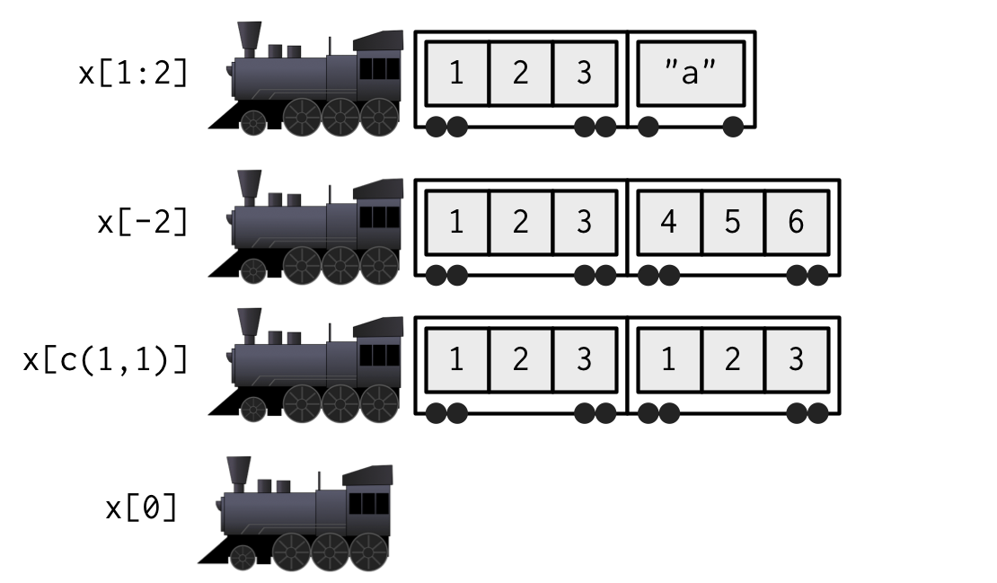
以提取atomic向量为例，介绍用作提取子集时的6种坐标：

x <- c(2.1, 4.2, 3.3, 5.4)

正整数：表示元素在向量中的位置。

x[c(3, 1)]
#> [1] 3.3 2.1
x[order(x)]
#> [1] 2.1 3.3 4.2 5.4

# Duplicate indices will duplicate values
x[c(1, 1)]
#> [1] 2.1 2.1

# Real numbers are silently truncated to integers
x[c(2.1, 2.9)]
#> [1] 4.2 4.2

负整数：负号表示删除，正负不能同时存在。

x[-c(3, 1)]
#> [1] 4.2 5.4


x[c(-1, 2)]
#> Error in x[c(-1, 2)]: only 0's may be mixed with negative subscripts

逻辑值：TRUE表示保留，FALSE表示删除，NA返回NA。在x[y]的模式中，如果二者长度不等，会发生循环，遵循R base中的循环原则：循环短的一方。

x[c(TRUE, TRUE, FALSE, FALSE)]
#> [1] 2.1 4.2
x[x > 3]
#> [1] 4.2 3.3 5.4
x[c(TRUE, NA, FALSE, TRUE)]
#> [1] 2.1  NA 5.4

Nothing：返回完整的对象，在后面对data.frame提取时有用。

x[]
#> [1] 2.1 4.2 3.3 5.4

Zero：返回长度为0的向量。

x[0]
#> numeric(0)

字符串：有name属性的向量元素。

(y <- setNames(x, letters[1:4]))
#>   a   b   c   d 
#> 2.1 4.2 3.3 5.4
y[c("d", "c", "a")]
#>   d   c   a 
#> 5.4 3.3 2.1

# Like integer indices, you can repeat indices
y[c("a", "a", "a")]
#>   a   a   a 
#> 2.1 2.1 2.1

# When subsetting with [, names are always matched exactly
z <- c(abc = 1, def = 2)
z[c("a", "d")]
#> <NA> <NA> 
#>   NA   NA

Note

不要使用因子化的字符串向量提取子集，字符串向量因子化后，会视为整数。

y[factor("b")]
#>   a 
#> 2.1

Lists

[函数作用于list时，返回得仍然是一个list；[[和$函数作用于list时，返回得是list中的元素。

Matrices and arrays

对于多维的atomic Vector，只需要在每个维度上应用上述6种坐标，就可以得到子集。

a <- matrix(1:9, nrow = 3)
colnames(a) <- c("A", "B", "C")
a[1:2, ]
#>      A B C
#> [1,] 1 4 7
#> [2,] 2 5 8
a[c(TRUE, FALSE, TRUE), c("B", "A")]
#>      B A
#> [1,] 4 1
#> [2,] 6 3
a[0, -2]
#>      A C

因为Matrices和Arrays是带有特殊属性的向量，所以仍然可以只使用一维的向量来提取，但要注意：它们都是列向量。

vals <- outer(1:5, 1:5, FUN = "paste", sep = ",")
vals
#>      [,1]  [,2]  [,3]  [,4]  [,5] 
#> [1,] "1,1" "1,2" "1,3" "1,4" "1,5"
#> [2,] "2,1" "2,2" "2,3" "2,4" "2,5"
#> [3,] "3,1" "3,2" "3,3" "3,4" "3,5"
#> [4,] "4,1" "4,2" "4,3" "4,4" "4,5"
#> [5,] "5,1" "5,2" "5,3" "5,4" "5,5"

vals[c(4, 15)]
#> [1] "4,1" "5,3"

可以使用一个两列matrix提取2维Matrices，三列matrix提取3维Arrays；一行表示一个坐标，返回一个向量。

select <- matrix(ncol = 2, byrow = TRUE, c(
  1, 1,
  3, 1,
  2, 4
))
select
#>      [,1] [,2]
#> [1,]    1    1
#> [2,]    3    1
#> [3,]    2    4
vals[select]
#> [1] "1,1" "3,1" "2,4"

Data frames and tibbles

Data.frame具有list和matrix的特性：

当只提供一个index时，会将其视作list，返回列。
当提供两个index时，将其视作matrix，返回矩阵。

df <- data.frame(x = 1:3, y = 3:1, z = letters[1:3])

df[df$x == 2, ]
#>   x y z
#> 2 2 2 b
df[c(1, 3), ]
#>   x y z
#> 1 1 3 a
#> 3 3 1 c

# There are two ways to select columns from a data frame
# Like a list
df[c("x", "z")]
#>   x z
#> 1 1 a
#> 2 2 b
#> 3 3 c

# Like a matrix
df[, c("x", "z")]
#>   x z
#> 1 1 a
#> 2 2 b
#> 3 3 c


# There's an important difference if you select a single
# column: matrix subsetting simplifies by default, list
# subsetting does not.
str(df["x"])
#> 'data.frame':    3 obs. of  1 variable:
#>  $ x: int  1 2 3
str(df[, "x"])
#>  int [1:3] 1 2 3

对tibble使用[，始终返回tibble。

tib <- tibble::tibble(x = 1:3, y = 3:1, z = letters[1:3])

str(tib["x"])
#> tibble [3 × 1] (S3: tbl_df/tbl/data.frame)
#>  $ x: int [1:3] 1 2 3
str(tib[, "x"])
#> tibble [3 × 1] (S3: tbl_df/tbl/data.frame)
#>  $ x: int [1:3] 1 2 3

Preserving dimensionality

[函数有额外的参数drop用于控制是否在只有一列时降维，默认为TRUE。

正如上面例子中的结果一样，data.frame在列方向上的index长度为1时，会发生降维：df["x"]没有发生降维，df[, "x"]则发生了降维。

str(df[, "x", drop = FALSE])
#> 'data.frame':    3 obs. of  1 variable:
#>  $ x: int  1 2 3

matrix则表现为任意维度的index长度为1时，都会发生降维：

a <- matrix(1:4, nrow = 2)
str(a[1, ])
#>  int [1:2] 1 3

str(a[1, , drop = FALSE])
#>  int [1, 1:2] 1 3

在factor中使用[时，也有参数drop；但该参数的意义为：是否丢弃没有值的级别，默认为FALSE。

z <- factor(c("a", "b"))
z[1]
#> [1] a
#> Levels: a b
z[1, drop = TRUE]
#> [1] a
#> Levels: a

Exercises

…

Selecting a single element

`[[`

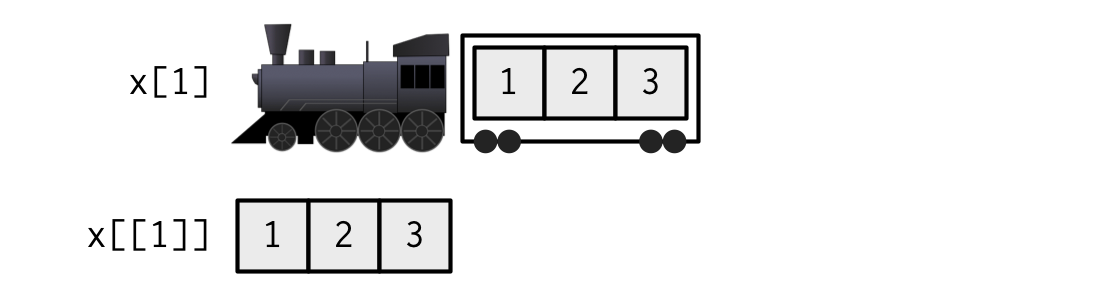
[[函数广泛应用在list或dataframe对象上，它与[函数的不同在于，返回得是降维的子对象。将一个list比作一列火车，[[返回的是火车中某车厢上的所有元素，[返回的是带有选取车厢的整列火车。

x <- list(1:3, "a", 4:6)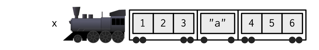

使用[[函数时要注意：

只能提供长度为1的整数或字符串作为index。
当提供的长度大于1后，会递归地提取子对象。

x1 <- list(
  1:3,
  list( "a", "b"),
  4:6
)

x1[[c(2,1)]]
#> [1] "a"
# 等价于
x1[[2]][[1]]
#> [1] "a"

`$`

x$y大致等于x[["y", exact = FALSE]]。

在使用$时，常见的错误是：使用当前环境变量中的某些变量来替代数据框或list中的name，此时推荐使用[[。

var <- "cyl"
# Doesn't work - mtcars$var translated to mtcars[["var"]]
mtcars$var
#> NULL

# Instead use [[
mtcars[[var]]
#>  [1] 6 6 4 6 8 6 8 4 4 6 6 8 8 8 8 8 8 4 4 4 4 8 8 8 8 4 4 4 8 6 8 4

$与[[最大的不同是，$会自动地执行从左到右地部分匹配；可以添加options(warnPartialMatchDollar = TRUE)来添加提醒。

x <- list(abc = 1)
x$a
#> [1] 1
x[["a"]]
#> NULL

options(warnPartialMatchDollar = TRUE)
x$a
#> Warning in x$a: partial match of 'a' to 'abc'
#> [1] 1

Missing and out-of-bounds indices

在使用[[函数时，如果index无效，不同类型对象的结果不同。如下表中总结，三种类型的数据：atomic向量，list和NULL，四种无效的index：长度为0，超出范围（整数、字符串），缺失。

row[[col]]	Zero-length	Out of bounds(Integer)	Out of bounds(character)	Missing
Atomic	Error	Error	Error	Error
List	Error	Error	NULL	NULL
NULL	NULL	NULL	NULL	NULL

x <- setNames(1:3, letters[1:3])
y <- list(A = 1:3, B = 4:6, C = 7:9)
z <- NULL

x[[NULL]]
x[[4]]
x[["d"]]
x[[NA]]

y[[NULL]]
y[[4]]
y[["D"]]
y[[NA]]

z[[NULL]]
z[[4]]
z[["D"]]
z[[NA]]

从表中可以看出，[[的结果存在非一致性。purrr包提供了另外两种取子集的函数purrr::pluck(),purrr::chuck()。purrr::pluck()可以设置元素缺失时的默认返回值（默认为NULL），purrr::chuck()总是返回错误。pluck()也允许混合整数和字符串的index。pluck()的优点，使得其在处理结构化数据json或web api结果时非常有用。

x <- list(
  a = list(1, 2, 3),
  b = list(3, 4, 5)
)

purrr::pluck(x, "a", 1)
#> [1] 1

purrr::pluck(x, "c", 1)
#> NULL

purrr::pluck(x, "c", 1, .default = NA)
#> [1] NA

`@` and `slot()`

@和slot()设计到S4面向对象系统，我们将在后面的章节中学习。

Exercises

…

Subsetting and assignment

查看函数说明文档，如果包含FUN(x) <-形式的函数，就支持赋值。

x <- 1:5
x[c(1, 2)] <- c(101, 102)
x
#> [1] 101 102   3   4   5

在使用赋值前，一定要检查好提取的子集长度等于赋的值长度、子集index唯一。因为base R的循环原则，会使得结果完全不符合预期。

对于list，可以使用x[[i]] <- NULL删除某个元素，如果是增加一个内容为NULL的元素可以使用x[i] <- list(NULL)。

x <- list(a = 1, b = 2)
x[["b"]] <- NULL
str(x)
#> List of 1
#>  $ a: num 1

y <- list(a = 1, b = 2)
y["b"] <- list(NULL)
str(y)
#> List of 2
#>  $ a: num 1
#>  $ b: NULL

前面讲到，提取空元素对atomic向量没有太多用处，但对数据框有重要作用：它可以保持数据框的数据结构：

mtcars[] <- lapply(mtcars, as.integer)
is.data.frame(mtcars)
#> [1] TRUE

mtcars <- lapply(mtcars, as.integer)
is.data.frame(mtcars)
#> [1] FALSE

Applications

利用取子集的功能，你可以对数据框进行查找、拼接、排序、抽样、解压、删除等操作，下面是一些应用广泛的例子：

Lookup tables (character subsetting)

创建查询表格，进行数据转换。

x <- c("m", "f", "u", "f", "f", "m", "m")
lookup <- c(m = "Male", f = "Female", u = NA)
lookup[x]
#>        m        f        u        f        f        m        m 
#>   "Male" "Female"       NA "Female" "Female"   "Male"   "Male"

# 去除name
unname(lookup[x])
#> [1] "Male"   "Female" NA       "Female" "Female" "Male"   "Male"

Matching and merging by hand (integer subsetting)

使用match()函数与整数索引进行数据匹配和合并。

grades <- c(1, 2, 2, 3, 1)

info <- data.frame(
  grade = 3:1,
  desc = c("Excellent", "Good", "Poor"),
  fail = c(F, F, T)
)

id <- match(grades, info$grade)
id
#> [1] 3 2 2 1 3
info[id, ]
#>     grade      desc  fail
#> 3       1      Poor  TRUE
#> 2       2      Good FALSE
#> 2.1     2      Good FALSE
#> 1       3 Excellent FALSE
#> 3.1     1      Poor  TRUE

Random samples and bootstraps (integer subsetting)

同上，使用整数索引，搭配sample()函数，模拟抽样与bootstrap。

df <- data.frame(x = c(1, 2, 3, 1, 2), y = 5:1, z = letters[1:5])

# Randomly reorder
df[sample(nrow(df)), ]
#>   x y z
#> 5 2 1 e
#> 3 3 3 c
#> 4 1 2 d
#> 1 1 5 a
#> 2 2 4 b

# Select 3 random rows
df[sample(nrow(df), 3), ]
#>   x y z
#> 4 1 2 d
#> 2 2 4 b
#> 1 1 5 a

# Select 6 bootstrap replicates
df[sample(nrow(df), 6, replace = TRUE), ]
#>     x y z
#> 5   2 1 e
#> 5.1 2 1 e
#> 5.2 2 1 e
#> 2   2 4 b
#> 3   3 3 c
#> 3.1 3 3 c

Ordering (integer subsetting)

同上，使用整数索引，搭配order()函数，对数据框排序。

# Randomly reorder df
df2 <- df[sample(nrow(df)), 3:1]
df2
#>   z y x
#> 5 e 1 2
#> 1 a 5 1
#> 4 d 2 1
#> 2 b 4 2
#> 3 c 3 3

df2[order(df2$x), ]
#>   z y x
#> 1 a 5 1
#> 4 d 2 1
#> 5 e 1 2
#> 2 b 4 2
#> 3 c 3 3
df2[, order(names(df2))]
#>   x y z
#> 5 2 1 e
#> 1 1 5 a
#> 4 1 2 d
#> 2 2 4 b
#> 3 3 3 c

Expanding aggregated counts (integer subsetting)

使用函数rep()，将行相同且具有重复数的数据框解压。

df <- data.frame(x = c(2, 4, 1), y = c(9, 11, 6), n = c(3, 5, 1))
rep(1:nrow(df), df$n)
#> [1] 1 1 1 2 2 2 2 2 3

df[rep(1:nrow(df), df$n), ]
#>     x  y n
#> 1   2  9 3
#> 1.1 2  9 3
#> 1.2 2  9 3
#> 2   4 11 5
#> 2.1 4 11 5
#> 2.2 4 11 5
#> 2.3 4 11 5
#> 2.4 4 11 5
#> 3   1  6 1

Removing columns from data frames (character)

删除数据框的某列。

df <- data.frame(x = 1:3, y = 3:1, z = letters[1:3])
df$z <- NULL

df <- data.frame(x = 1:3, y = 3:1, z = letters[1:3])
df[c("x", "y")]
#>   x y
#> 1 1 3
#> 2 2 2
#> 3 3 1

df[setdiff(names(df), "z")]
#>   x y
#> 1 1 3
#> 2 2 2
#> 3 3 1

Selecting rows based on a condition (logical subsetting)

使用逻辑向量筛选数据框的行。

data(mtcars)
mtcars[mtcars$gear == 5, ]
#>                 mpg cyl  disp  hp drat    wt qsec vs am gear carb
#> Porsche 914-2  26.0   4 120.3  91 4.43 2.140 16.7  0  1    5    2
#> Lotus Europa   30.4   4  95.1 113 3.77 1.513 16.9  1  1    5    2
#> Ford Pantera L 15.8   8 351.0 264 4.22 3.170 14.5  0  1    5    4
#> Ferrari Dino   19.7   6 145.0 175 3.62 2.770 15.5  0  1    5    6
#> Maserati Bora  15.0   8 301.0 335 3.54 3.570 14.6  0  1    5    8

mtcars[mtcars$gear == 5 & mtcars$cyl == 4, ]
#>                mpg cyl  disp  hp drat    wt qsec vs am gear carb
#> Porsche 914-2 26.0   4 120.3  91 4.43 2.140 16.7  0  1    5    2
#> Lotus Europa  30.4   4  95.1 113 3.77 1.513 16.9  1  1    5    2

Boolean algebra versus sets (logical and integer )

which()函数可以将布尔索引转换为整数索引。但x[which(y)]与x[y]仍然有一些差别：

当布尔索引中存在缺失值NA时，对应得返回值也是NA。而which()会自动丢掉NA。
x[-which(y)]与x[!y]不是等价的：如有y全部是FALSE，which(y)返回integer(0)，而-integer(0)仍然是integer(0)，最终前者返回一个空的向量，后者返回全部值。

x <- c(1, 2, 3, 4, NA, 5)

x[which(x > 2)]
#> [1] 3 4 5
x[x > 2]
#> [1]  3  4 NA  5

x[-which(x > 10)]
#> numeric(0)
x[!x > 10]
#> [1]  1  2  3  4 NA  5

布尔向量的运算可以使用intersect()，`union()，setdiff()等函数进行等价替换。

(x1 <- 1:10 %% 2 == 0)
#>  [1] FALSE  TRUE FALSE  TRUE FALSE  TRUE FALSE  TRUE FALSE  TRUE
(x2 <- which(x1))
#> [1]  2  4  6  8 10
(y1 <- 1:10 %% 5 == 0)
#>  [1] FALSE FALSE FALSE FALSE  TRUE FALSE FALSE FALSE FALSE  TRUE
(y2 <- which(y1))
#> [1]  5 10

# X & Y <-> intersect(x, y)
x1 & y1
#>  [1] FALSE FALSE FALSE FALSE FALSE FALSE FALSE FALSE FALSE  TRUE
intersect(x2, y2)
#> [1] 10

# X | Y <-> union(x, y)
x1 | y1
#>  [1] FALSE  TRUE FALSE  TRUE  TRUE  TRUE FALSE  TRUE FALSE  TRUE
union(x2, y2)
#> [1]  2  4  6  8 10  5

# X & !Y <-> setdiff(x, y)
x1 & !y1
#>  [1] FALSE  TRUE FALSE  TRUE FALSE  TRUE FALSE  TRUE FALSE FALSE
setdiff(x2, y2)
#> [1] 2 4 6 8

# xor(X, Y) <-> setdiff(union(x, y), intersect(x, y))
xor(x1, y1)
#>  [1] FALSE  TRUE FALSE  TRUE  TRUE  TRUE FALSE  TRUE FALSE FALSE
setdiff(union(x2, y2), intersect(x2, y2))
#> [1] 2 4 6 8 5

Introduction

Outline

Selecting multiple elements

Atomic vectors

Lists

Matrices and arrays

Data frames and tibbles

Preserving dimensionality

Exercises

Selecting a single element

[[

$

Missing and out-of-bounds indices

@ and slot()

Exercises

Subsetting and assignment

Applications

Lookup tables (character subsetting)

Matching and merging by hand (integer subsetting)

Random samples and bootstraps (integer subsetting)

Ordering (integer subsetting)

Expanding aggregated counts (integer subsetting)

Removing columns from data frames (character)

Selecting rows based on a condition (logical subsetting)

Boolean algebra versus sets (logical and integer )

`[[`

`$`

`@` and `slot()`